---

In a presentation to a group of aerospace engineers on the differences between calibration and tuning, I explained that both involve solving inverse problems but differ fundamentally in their objectives, methodologies, and scope.

• Calibration aims to determine material property coefficients (e.g., elastic moduli, proportional limit, thermal conductivity, permeability) and other relationships such as the dependence of crack-growth increment on stress-intensity factor. These quantities are inferred from measurements. Load-displacement responses or cycles-to-crack-length data are examples. The inferences rely on the numerical solution of a well-posed mathematical problem. It is essential that the approximation error in the quantities of interest be negligibly small compared with the observational errors.
• Tuning, in contrast, aims to adjust stiffness relationships in finite element models to match experimentally determined force-displacement curves, or to determine the internal force distribution in an aircraft structural load model, or the energy absorption characteristics of a vehicle in crash analysis. In this process, the resulting numerical problem does not need to be (and usually is not) an approximation to any well‑posed mathematical problem. Consequently, it is not meaningful to speak of errors of approximation.

The Domain of Calibration (DoC)

In the calibration process, inferences are drawn from experimental data. Inevitably, these data are only available over limited intervals. Additional restrictions on the admissible data arise from the assumptions incorporated into the mathematical model, such as small-strain or small-deformation kinematics, nonlinear material laws, the deformation theory of plasticity, requirements on the regularity of material properties, and the applied loads. The set of restrictions on the calibration parameters and admissible data constitutes the domain of calibration [1]. A model can make reliable predictions only when the input data and parameters are within the domain of calibration. In other words, a model is validated with respect to its domain of calibration.

An important goal of model development is to ensure that the domain of calibration is sufficiently large to cover all intended applications of the model.

The Domain of Tuning (DoT)

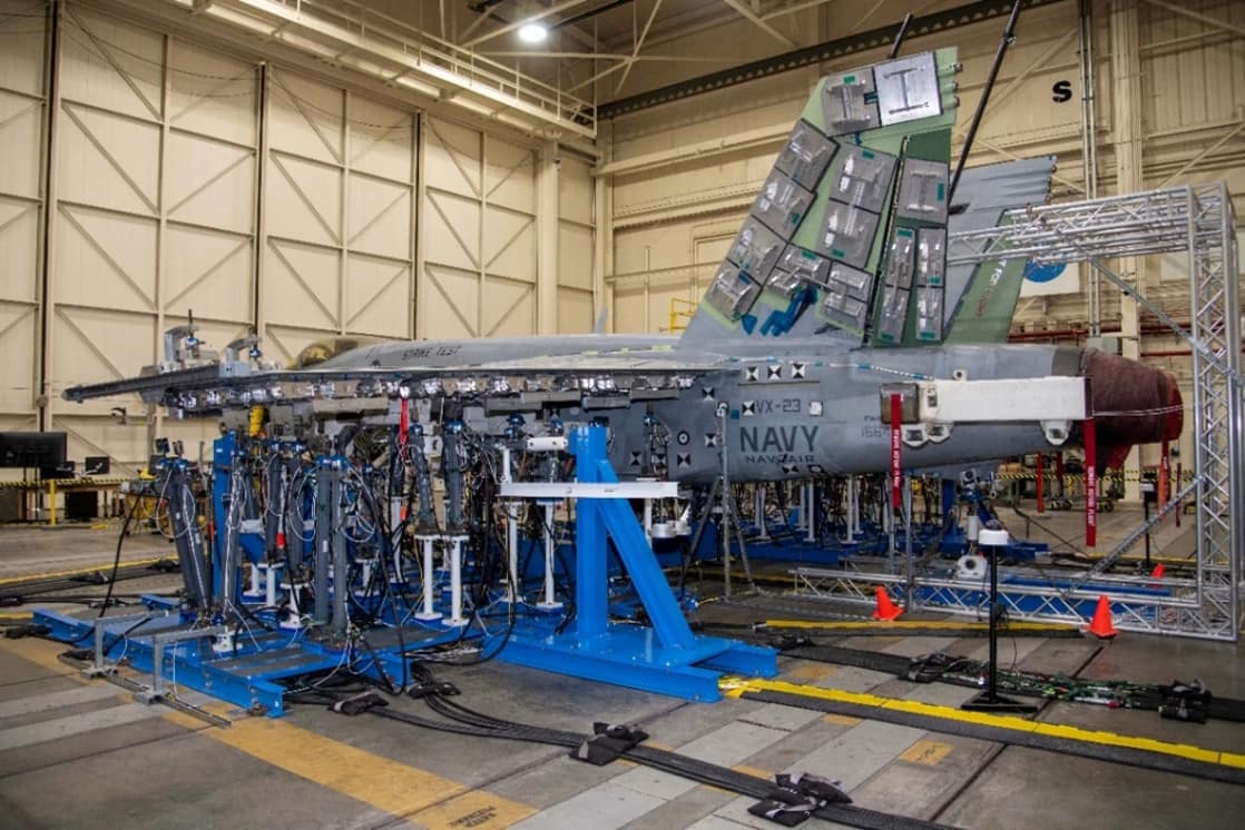
In finite element modeling, elements are selected from the element library of a legacy finite element software product to approximate the geometric configuration of a structure, such as an airframe, vehicle body, ship hull, or some other structure. Material properties are then assigned to these elements to represent the stiffness—or, more generally, the load-displacement characteristics—of structural components such as the keel, bulkheads, spars, ribs, and skin. Various shortcuts, such as point constraints and reduced integration, which fall into the category of variational crimes, are usually employed in this process. The goal is to estimate the distribution of internal forces corresponding to the load cases considered in the design. See, for example, [2].

If n adjustable parameters characterize the model, then tuning produces a point in an n-dimensional parameter space. The domain of tuning degenerates to this point. When models are developed for vehicles of different designs, they form a cluster of points in this space. The domain of tuning is this set of points. It is then possible, with many caveats, to predict the crash dynamics of a previously untested design by interpolating between these known points [3]. These caveats primarily stem from the high non-linearity of irreversible structural deformation and the sparsity of data in high-dimensional spaces, which contribute to interpolation errors.

Proper Uses of Tuned Models

Tuned finite element models play an important role in numerical simulation. A complex structure, such as an airframe, is modeled at length scales ranging from tens of meters to the size of the representative volume element (RVE) for the material. 

By definition, an RVE is the smallest volume of a material that is statistically representative of the overall macroscopic properties of an entire structure. The average values of material properties such as elastic modulus, thermal conductivity, permeability, over this volume, yield values that closely approximate those of the bulk material. In the case of aluminum, the diameter of RVE is roughly one millimeter.

 For example, an aircraft structure is typically partitioned into the following levels:

1. Airframe: The complete, integrated structural skeleton of the aircraft.
2. Assemblies: The primary sections of the aircraft, such as the wing, the fuselage, and the empennage.
3. Sub-assemblies: Larger integrated units that perform major structural or aerodynamic roles, such as a wing trailing edge, a nose‑cone section, or a flap.
4. Components: Collections of parts joined together to perform a specific structural function, such as a built-up spar or a window frame.
5. Sub-components: Individual fabricated items made from a single piece of material, such as a rib, a section of a stringer, or a bracket.

The subcomponents and components are designed for strength and durability, which requires solving well-posed mathematical problems whose accuracy depends, in part, on the boundary conditions derived from tuned models of higher-level assemblies. Multi-scale simulations can be visualized as a chain; the first link is the load model of the entire structure, such as an airframe, followed by assemblies, subassemblies, components, and subcomponents. The reliability of predictions depends on the weakest link in this chain. The first three links typically rely on tuned finite element models, while the last two rely on calibrated mathematical models.

Improper Uses of Tuned Models

It would be improper to use a tuned finite element model to predict quantities of interest that depend on derivatives of the displacement field, such as strains, stresses, and stress intensity factors. These quantities lie outside the scope of tuning.

The Limitations of Tuning

Following the presentation, one of the attendees told me that the explanation of tuning reminded him of a story from the early days of color television:

Two engineers were testing a new color TV link—one at the studio with a camera pointed at a bowl of fruit, the other miles away at the receiver, adjusting the settings for color balance over the phone. On the morning of April 1, the engineer in the studio painted the banana purple and waited.

Hours later, the phone rang. His colleague at the receiver, greatly agitated, said, “I don’t know what’s going on. I’ve finally gotten the banana looking right, but now everything else is wrong!”

This story sums up the limitations of tuning very well.

---

References

[1] Szabó, B. and Actis, R. The demarcation problem in the applied sciences. Computers & Mathematics with Applications, 162, pp. 206-214, 2024.

[2] Mottershead, J.E. and Friswell, M.I. Model updating in structural dynamics: a survey. Journal of sound and vibration, 167(2), pp. 347-375, 1993.

[3] Bayarri, M.J., Berger, J.O., Kennedy, M.C., Kottas, A., Paulo, R., Sacks, J., Cafeo, J.A., Lin, C.H. and Tu, J. Predicting vehicle crashworthiness: Validation of computer models for functional and hierarchical data. Journal of the American Statistical Association, 104(487), pp. 929-943, 2009.

---

Related Blogs:

• A Memo from the 5th Century BC
• Obstacles to Progress
• Why Finite Element Modeling is Not Numerical Simulation?
• XAI Will Force Clear Thinking About the Nature of Mathematical Models
• The Story of the P-version in a Nutshell
• Why Worry About Singularities?
• Questions About Singularities
• A Low-Hanging Fruit: Smart Engineering Simulation Applications
• The Demarcation Problem in the Engineering Sciences
• Model Development in the Engineering Sciences
• Certification by Analysis (CbA) – Are We There Yet?
• Not All Models Are Wrong
• Digital Twins
• Digital Transformation
• Simulation Governance
• Variational Crimes
• The Kuhn Cycle in the Engineering Sciences
• Finite Element Libraries: Mixing the “What” with the “How”
• A Critique of the World Wide Failure Exercise
• Meshless Methods
• Isogeometric Analysis (IGA)
• Chaos in the Brickyard Revisited
• Why Is Solution Verification Necessary?
• Variational Crimes and Refloating the Costa Concordia
• Lessons From a Failed Model Development Project
• Where Do You Get the Courage to Sign the Blueprint?
• Great Expectations: Agentic AI in Mechanical Engineering